Note
Click here to download the full example code
Train, convert and predict with ONNX Runtime
This example demonstrates an end to end scenario starting with the training of a machine learned model to its use in its converted from.
Train a logistic regression
The first step consists in retrieving the iris datset.
from sklearn.datasets import load_iris
iris = load_iris()
X, y = iris.data, iris.target

from sklearn.model_selection import train_test_split
X_train, X_test, y_train, y_test = train_test_split(X, y)
Then we fit a model.
from sklearn.linear_model import LogisticRegression
clr = LogisticRegression()
clr.fit(X_train, y_train)
Out:
/home/runner/.local/lib/python3.8/site-packages/sklearn/linear_model/_logistic.py:814: ConvergenceWarning: lbfgs failed to converge (status=1):
STOP: TOTAL NO. of ITERATIONS REACHED LIMIT.

Increase the number of iterations (max_iter) or scale the data as shown in:
    https://scikit-learn.org/stable/modules/preprocessing.html
Please also refer to the documentation for alternative solver options:
    https://scikit-learn.org/stable/modules/linear_model.html#logistic-regression
  n_iter_i = _check_optimize_result(

LogisticRegression()
We compute the prediction on the test set and we show the confusion matrix.
from sklearn.metrics import confusion_matrix

pred = clr.predict(X_test)
print(confusion_matrix(y_test, pred))
Out:
[[12  0  0]
 [ 0 14  0]
 [ 0  1 11]]
Conversion to ONNX format
We use module sklearn-onnx to convert the model into ONNX format.
from skl2onnx import convert_sklearn
from skl2onnx.common.data_types import FloatTensorType

initial_type = [('float_input', FloatTensorType([None, 4]))]
onx = convert_sklearn(clr, initial_types=initial_type)
with open("logreg_iris.onnx", "wb") as f:
    f.write(onx.SerializeToString())
We load the model with ONNX Runtime and look at its input and output.
import onnxruntime as rt
sess = rt.InferenceSession("logreg_iris.onnx", providers=rt.get_available_providers())

print("input name='{}' and shape={}".format(
    sess.get_inputs()[0].name, sess.get_inputs()[0].shape))
print("output name='{}' and shape={}".format(
    sess.get_outputs()[0].name, sess.get_outputs()[0].shape))
Out:
input name='float_input' and shape=[None, 4]
output name='output_label' and shape=[None]
We compute the predictions.
input_name = sess.get_inputs()[0].name
label_name = sess.get_outputs()[0].name

import numpy
pred_onx = sess.run([label_name], {input_name: X_test.astype(numpy.float32)})[0]
print(confusion_matrix(pred, pred_onx))
Out:
[[12  0  0]
 [ 0 15  0]
 [ 0  0 11]]
The prediction are perfectly identical.
Probabilities
Probabilities are needed to compute other relevant metrics such as the ROC Curve. Let’s see how to get them first with scikit-learn.
prob_sklearn = clr.predict_proba(X_test)
print(prob_sklearn[:3])
Out:
[[1.62238218e-02 7.68683337e-01 2.15092842e-01]
 [2.11069571e-03 4.12946172e-01 5.84943132e-01]
 [9.71843891e-01 2.81559619e-02 1.46792565e-07]]
And then with ONNX Runtime. The probabilies appear to be
prob_name = sess.get_outputs()[1].name
prob_rt = sess.run([prob_name], {input_name: X_test.astype(numpy.float32)})[0]

import pprint
pprint.pprint(prob_rt[0:3])
Out:
[{0: 0.016223827376961708, 1: 0.7686832547187805, 2: 0.21509289741516113},
 {0: 0.0021106956992298365, 1: 0.4129459857940674, 2: 0.5849433541297913},
 {0: 0.9718438386917114, 1: 0.02815595641732216, 2: 1.467925159204242e-07}]
Let’s benchmark.
from timeit import Timer

def speed(inst, number=10, repeat=20):
    timer = Timer(inst, globals=globals())
    raw = numpy.array(timer.repeat(repeat, number=number))
    ave = raw.sum() / len(raw) / number
    mi, ma = raw.min() / number, raw.max() / number
    print("Average %1.3g min=%1.3g max=%1.3g" % (ave, mi, ma))
    return ave

print("Execution time for clr.predict")
speed("clr.predict(X_test)")

print("Execution time for ONNX Runtime")
speed("sess.run([label_name], {input_name: X_test.astype(numpy.float32)})[0]")
Out:
Execution time for clr.predict
Average 7.16e-05 min=6.55e-05 max=8.98e-05
Execution time for ONNX Runtime
Average 3.89e-05 min=2.54e-05 max=6.37e-05

3.893253500052652e-05
Let’s benchmark a scenario similar to what a webservice experiences: the model has to do one prediction at a time as opposed to a batch of prediction.
def loop(X_test, fct, n=None):
    nrow = X_test.shape[0]
    if n is None:
        n = nrow
    for i in range(0, n):
        im = i % nrow
        fct(X_test[im: im+1])

print("Execution time for clr.predict")
speed("loop(X_test, clr.predict, 100)")

def sess_predict(x):
    return sess.run([label_name], {input_name: x.astype(numpy.float32)})[0]

print("Execution time for sess_predict")
speed("loop(X_test, sess_predict, 100)")
Out:
Execution time for clr.predict
Average 0.00625 min=0.00577 max=0.00722
Execution time for sess_predict
Average 0.00141 min=0.00132 max=0.00162

0.0014080239099996561
Let’s do the same for the probabilities.
print("Execution time for predict_proba")
speed("loop(X_test, clr.predict_proba, 100)")

def sess_predict_proba(x):
    return sess.run([prob_name], {input_name: x.astype(numpy.float32)})[0]

print("Execution time for sess_predict_proba")
speed("loop(X_test, sess_predict_proba, 100)")
Out:
Execution time for predict_proba
Average 0.00944 min=0.00855 max=0.011
Execution time for sess_predict_proba
Average 0.00161 min=0.00132 max=0.00206

0.0016082661699991264
This second comparison is better as ONNX Runtime, in this experience, computes the label and the probabilities in every case.
Benchmark with RandomForest
We first train and save a model in ONNX format.
from sklearn.ensemble import RandomForestClassifier
rf = RandomForestClassifier()
rf.fit(X_train, y_train)

initial_type = [('float_input', FloatTensorType([1, 4]))]
onx = convert_sklearn(rf, initial_types=initial_type)
with open("rf_iris.onnx", "wb") as f:
    f.write(onx.SerializeToString())
We compare.
sess = rt.InferenceSession("rf_iris.onnx", providers=rt.get_available_providers())

def sess_predict_proba_rf(x):
    return sess.run([prob_name], {input_name: x.astype(numpy.float32)})[0]

print("Execution time for predict_proba")
speed("loop(X_test, rf.predict_proba, 100)")

print("Execution time for sess_predict_proba")
speed("loop(X_test, sess_predict_proba_rf, 100)")
Out:
Execution time for predict_proba
Average 1.19 min=1.16 max=1.23
Execution time for sess_predict_proba
Average 0.00197 min=0.00177 max=0.00237

0.0019650150299986534
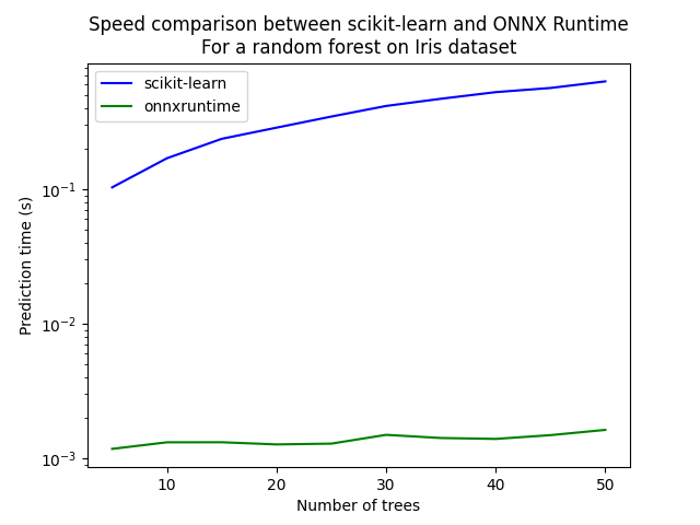
Let’s see with different number of trees.
measures = []

for n_trees in range(5, 51, 5):
    print(n_trees)
    rf = RandomForestClassifier(n_estimators=n_trees)
    rf.fit(X_train, y_train)
    initial_type = [('float_input', FloatTensorType([1, 4]))]
    onx = convert_sklearn(rf, initial_types=initial_type)
    with open("rf_iris_%d.onnx" % n_trees, "wb") as f:
        f.write(onx.SerializeToString())
    sess = rt.InferenceSession("rf_iris_%d.onnx" % n_trees, providers=rt.get_available_providers())
    def sess_predict_proba_loop(x):
        return sess.run([prob_name], {input_name: x.astype(numpy.float32)})[0]
    tsk = speed("loop(X_test, rf.predict_proba, 100)", number=5, repeat=5)
    trt = speed("loop(X_test, sess_predict_proba_loop, 100)", number=5, repeat=5)
    measures.append({'n_trees': n_trees, 'sklearn': tsk, 'rt': trt})

from pandas import DataFrame
df = DataFrame(measures)
ax = df.plot(x="n_trees", y="sklearn", label="scikit-learn", c="blue", logy=True)
df.plot(x="n_trees", y="rt", label="onnxruntime",
                ax=ax, c="green", logy=True)
ax.set_xlabel("Number of trees")
ax.set_ylabel("Prediction time (s)")
ax.set_title("Speed comparison between scikit-learn and ONNX Runtime\nFor a random forest on Iris dataset")
ax.legend()
Out:
5
Average 0.103 min=0.102 max=0.105
Average 0.00117 min=0.00106 max=0.00124
10
Average 0.17 min=0.164 max=0.175
Average 0.00131 min=0.00125 max=0.00142
15
Average 0.237 min=0.232 max=0.242
Average 0.00131 min=0.00114 max=0.00146
20
Average 0.287 min=0.28 max=0.292
Average 0.00127 min=0.00112 max=0.00149
25
Average 0.347 min=0.342 max=0.354
Average 0.00128 min=0.00114 max=0.00157
30
Average 0.416 min=0.414 max=0.424
Average 0.00149 min=0.00134 max=0.00157
35
Average 0.471 min=0.458 max=0.487
Average 0.00141 min=0.0013 max=0.00146
40
Average 0.527 min=0.511 max=0.534
Average 0.00139 min=0.00123 max=0.00165
45
Average 0.566 min=0.55 max=0.586
Average 0.00148 min=0.00138 max=0.00172
50
Average 0.634 min=0.611 max=0.647
Average 0.00162 min=0.00141 max=0.00189

<matplotlib.legend.Legend object at 0x7f8dccbc8460>
Total running time of the script: ( 5 minutes 38.359 seconds)